Endophenotypes
Each subject in the study group was assessed for 12 endophenotypes, as described elsewhere in detail (
13,
14), all of which have been shown to be heritable (
15). Prepulse inhibition was measured as the percentage inhibition of the startle reflex in response to a weak prestimulus with a 60-msec interval from prepulse to startle stimulus (
16–
18). P50 suppression was measured as the difference between the amplitudes of the P50 event-related potentials generated in response to conditioning and test stimuli presented with a 500-msec interstimulus interval (
19,
20). Although the ratio is the more commonly used measure of P50 suppression, we have found the difference score to be more heritable in our COGS families (
15). The “overlap” antisaccade task of oculomotor inhibition, which requires subjects to fixate on a central target and respond to a peripheral cue by looking in the opposite direction at the same distance, was measured as the ratio of correct antisaccades to total interpretable saccades (
21,
22). The degraded stimulus version of the Continuous Performance Test (referred to later as “continuous performance”), a widely used measure of deficits in sustained, focused attention with a high perceptual load, was used to assess correct target detections and incorrect responses to nontargets (d′) (
23 and 1999 software by K.H. Nuechterlein and R.F. Asarnow, version 8.11). The letter-number span, part of the Wechsler Memory Scale, is a prototypical task to assess storage of working memory information with manipulation; it requires the correct reordering of intermixed numbers and letters. For the assessment of verbal learning and memory, we used the California Verbal Learning Test (
24) (“verbal learning”), an established list-learning test that provides a total score for recall of a list of 16 verbally presented items summed over five trials.
We also employed a modified version of the University of Pennsylvania Computerized Neurocognitive Battery (
25,
26), excluding measures of attention and verbal and working memory, which were assessed as detailed in the preceding. Six measures were evaluated by using this battery. The test for abstraction and mental flexibility (“abstraction”) presents four objects from which the subject must choose the one that does not belong. An assessment of face memory requires subjects to recognize 20 previously presented target faces among 20 distracter faces. The assessment of spatial memory uses euclidean shapes as learning stimuli in a recognition paradigm identical to that used for face memory. For an assessment of spatial processing, two lines are presented at an angle, and the corresponding lines must be identified on a simultaneously presented array. The assessment of sensorimotor dexterity requires the subject to click with a mouse as quickly as possible on a target that gets increasingly smaller. The assessment of emotion recognition involves the correct identification of a variety of facial expressions of emotion. Each of these tests was measured as “efficiency,” calculated as accuracy/(log
10 speed) and expressed as standard equivalents (z scores).
Custom SNP Chip
Genes of interest were identified and ranked in terms of their level of importance in understanding schizophrenia according to complementary information from a number of research domains: 1) linkage and association studies of schizophrenia and related phenotypes, 2) model organism, gene expression, and brain imaging studies, and 3) genetic networks and biological pathways relevant to schizophrenia. We mined public databases for general information about the genes and polymorphic variants of interest, including haplotype-tagging and potentially functional SNPs and those with previous reports of association with schizophrenia or related phenotypes. These data were then combined and compared to the list of SNPs available from Illumina, Inc. (San Diego, Calif.), for choice of the final 1,536 SNPs in 94 genes. A total of 1,417 haplotype-tagging SNPs obtained from the TAMAL web site (Technology And Money Are Limiting;
27) were selected from Caucasian HapMap populations (
28) to efficiently interrogate 86 of the genes with an r
2 threshold of 0.8 in our primarily (89%) Caucasian subjects. We included 5 kilobases (kb) of flanking sequence on either side of each gene to capture nearby regulatory elements in the tagged regions. The TAGGER SNP selection algorithm (
29), with an aggressive tagging mode forcing all coding SNPs into the model, was used to select tagging SNPs for 76 of the genes. The SNP selection algorithm of Gabriel et al. (
30) with a pairwise tagging mode was used to select tagging SNPs for an additional 10 genes to achieve sufficient gene coverage with the available SNPs. A combination of gene-spanning and putatively associated SNPs was used for the remaining eight genes because suitable tagging SNPs were not available. For CHRNA7, SNPs were selected within exons/introns 1–4 only, as the remainder of the gene cannot be screened because of a partial duplication, CHRFAM7A (
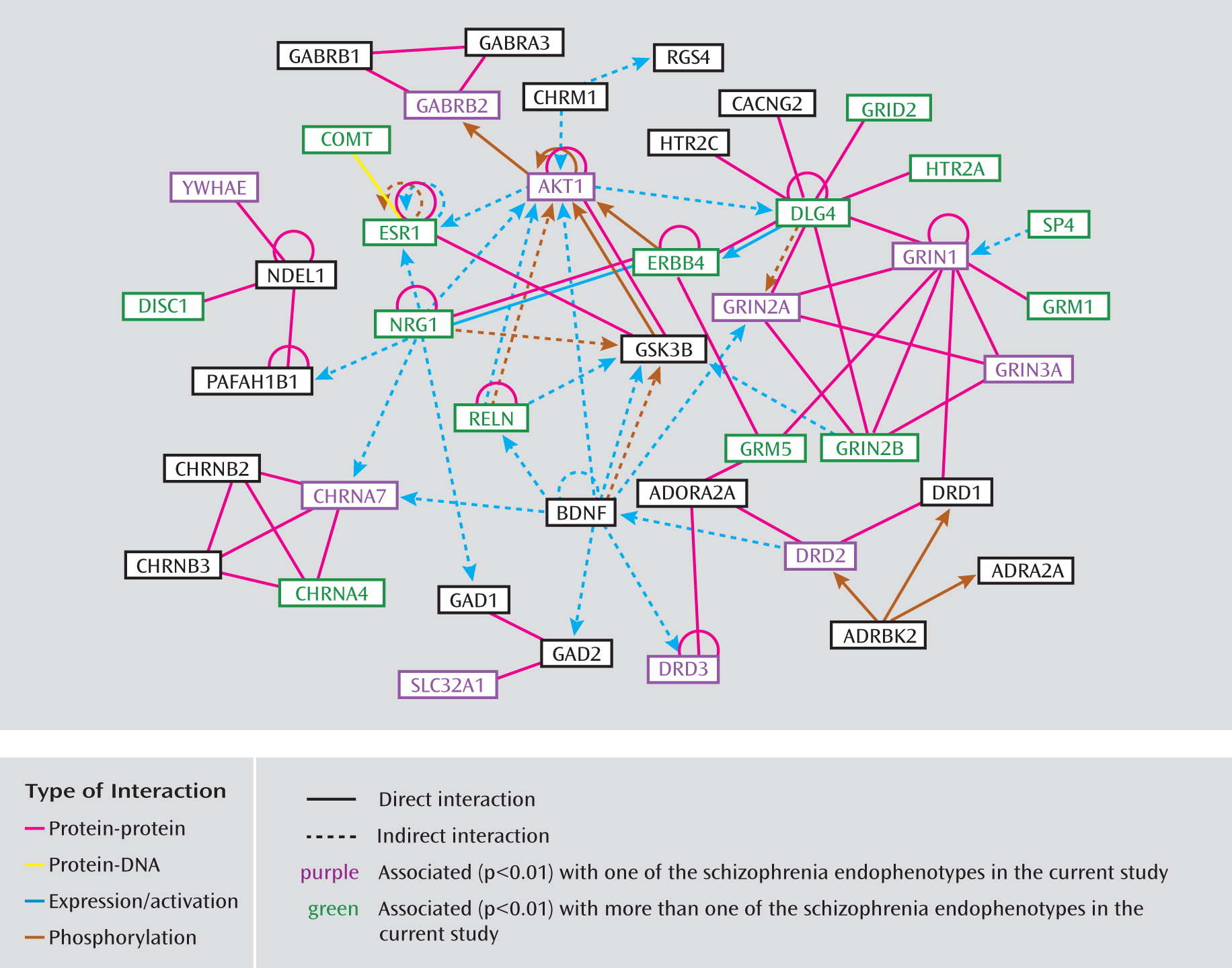
31). The custom array includes 109 SNPs in 33 genes with reported evidence of association, 29 coding sequence variants in 17 genes (25 nonsynonymous and four synonymous), and 18 SNPs located in putative promoter regions or transcription factor binding sites. On average, there is one SNP per 10 kb for each gene with variance due to linkage disequilibrium patterns, SNP availability, etc. Minor allele frequencies for these SNPs ranged from 0.01 to 0.50, with an average of 0.23. The complete list of all 1,536 SNPs and 94 candidate genes included on the COGS SNP chip and the specific details from our research are available in Supplemental Table 1, which accompanies the online version of this article; this information includes RefSNP accession identification numbers (rs numbers), chromosomal locations, gene information, designation of SNPs (e.g., as tagging, coding, putatively functional, or associated, including p values and references), relevant sequence information, and minor allele frequencies for the four HapMap populations. Ingenuity Pathway Analysis (Ingenuity Systems, Redwood City, Calif.) was used to investigate the molecular interactions among the included genes and to provide information regarding pathway membership.
Total Significance Test for Multiple Tests
To test whether the observed genotype-endophenotype associations significantly exceed what would be seen by chance given that there are 16,620 total tests (1,385 SNPs and 12 endophenotypes), we developed and implemented a separate, novel multiple testing strategy, the bootstrap total significance test. Our strategy introduces two innovations that together overcome several limitations of existing genomic multiple testing methods.
First, we base our approach on bootstrap sampling instead of permutation sampling. The bootstrap works in settings where permutation tests cannot be applied or can be applied only with difficulty (
36). Bootstrapping allows straightforward handling of family data even with complex patterns of missing data. In contrast, permutation procedures for family data are difficult to construct and do not use all information in the data if genetic variants drive phenotypic differences between families (
36). Bootstrapping also handles confounding variables easily. Permutation tests do not, as the confounder is potentially associated with both predictor and outcome under the null hypothesis. Most important, this problem arises when covariates are included to adjust for cryptic population stratification. Bootstrapping will also work when the goal is to test an interaction in the presence of main effects.
Second, we introduce the concept of a total significance test to determine whether the strongest genotype-endophenotype associations are more extreme than expected by chance alone. The total significance test provides a rigorous statistical p value that collectively applies to the strongest results in the data but is less conservative than standard p value adjustments for multiple tests. This test is less dependent than other multiple testing methods on extremely small p values, which are difficult to obtain with moderate group sizes and may, even in large groups, be due more to rare sampling events or statistical flukes than to replicable biological findings. Last, we use the results of the bootstrap total significance test to provide an a posteriori predictive value for each genotype-endophenotype association, giving a measure of how likely each detected association is to be true. When the preceding factors are not present and bootstrapping is not required, the total significance test can also be based on permutation sampling.
We implemented the bootstrap total significance test in MatLab (MathWorks, Natick, Mass.). Specifically, we first applied a multiple regression model to the original data for each of the 1,385×12 SNP-endophenotype combinations, with the endophenotype as the dependent variable and the SNP (coded as the number of copies of the minor allele) and relevant covariates (those used in the variance-component Merlin analyses) as independent predictors. Thus, the multiple regression model used in the total significance test was identical to the variance-component model used in the Merlin analyses, with the sole exception of the within-family correlation structure. For each SNP-endophenotype combination in the original data, we calculated a z statistic, Z=(B–0)/s, where B is the estimated regression coefficient corresponding to the SNP and s is its estimated standard error (SE) in the multiple regression. The value 0 is the expected value of B under the null hypothesis of no SNP-endophenotype association.
We then simulated the same statistics under the null hypothesis by generating one group of 10,000 random bootstrap data sets (the training group) and a second group of 1,000 identically generated bootstrap data sets (the test group), following standard bootstrap theory for clustered data (
37). To create each bootstrap data set, we randomly selected families from the original set of 130 families with replacement (i.e., families were selected randomly without respect to whether they were previously selected). Any one of the original families can appear multiple times in a single bootstrap data set or not at all. Each time a family appears, all data associated with it are placed in the new data set, including all family members, their covariates, endophenotypes, and genotypes. No data are rearranged, as they would be in a permutation test. For each bootstrap data set, z statistics were calculated as Z*=(B*–B)/s*, where
B* and
s* are the regression coefficient and SE calculated from the multiple regression applied to the bootstrap data. For a bootstrap sample, the true null hypothesis is given by the value estimated in the original data set, so that
B replaces 0 in the formula for
Z. The bootstrap
Z* values provide an empirical estimate of the joint distribution of the
Z values in the original data set, under the null hypothesis of no association. This is an application of standard bootstrap theory that is used, for example, in construction of the bootstrap-t confidence interval (
37). The bootstrap automatically incorporates the empirically observed family-level correlation structure without relying on the assumption of a multivariate normal distribution, as well as inter-SNP correlations due to linkage disequilibrium.
To evaluate the p value for the total significance test, we then compared the test statistics for the original data to their bootstrap distributions. For each Z, we evaluated whether it was so extreme as to fall outside the range of Z* values for the same SNP-endophenotype combination in the 10,000 training bootstrap data sets. As each SNP-endophenotype combination is compared to its own distinct bootstrap distribution, an advantage of our approach is that there is no implicit assumption about exchangeability or identically distributed SNPs or endophenotypes. Let T0 be the total number of tested associations in the original data for which Z is either less than the minimum Z* or more than the maximum Z* in the 10,000 data set training group. Similarly, let T0* be the total number for each of the 1,000 independent bootstrap data sets in the test group, also based on comparison to the 10,000 data set training group. The collective p value for T0 is the proportion of bootstrap test data sets for which T0*≥T0. The question addressed by the total significance test is different from that for the “no family-wise error” criterion provided by a Bonferroni correction or a traditional permutation test. Thus, p values from the total significance test are not comparable to those provided by these other methods.
To obtain a posterior predictive value for the associations that were so significant as to be outside the range of the training group, we calculated the expected number of false positives F0 at this level as the averageT0* in the 1,000 training data sets. The posterior predictive value for all associations in this initial group was then calculated as (R0–F0)/R0, where R0 is the number actually out of range in the original data.
We then extended this approach to determine if somewhat weaker results, those within the range of the tails of the bootstrap distribution, also significantly exceeded results expected by chance. Let T1 and T1* refer to totals based on comparison to the training group after the smallest and largest Z* values for each SNP-endophenotype combination are discarded. The subscript denotes the number discarded. A cumulative p value for T1 was calculated as the proportion of bootstrap data sets in the test group for which either T1*≥T1, T0*≥ T0, or both. T2, T3, and so on were computed, and a cumulative p value was calculated for each, with consideration of all prior tests of greater stringency. This p value simultaneously accounts for all stronger results and must increase sequentially. We considered all results satisfying a total cumulative, collective p value of ≤0.05 to be significant by the total significance and calculated posterior predictive values for each analogous to those described in the preceding.
