Acute Treatment Protocols
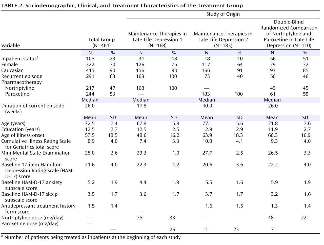
During the acute phase of maintenance therapies in late-life depression, the subjects were treated openly with nortriptyline titrated to yield a plasma level of 80–120 ng/ml, combined with weekly interpersonal therapy. During the acute phase of treatment in maintenance therapies in late-life depression 2, the subjects were treated openly with paroxetine in doses adjusted between 10 and 40 mg/day based on tolerability and response (mean [SD] final dose: 26 [11] mg/day), combined with weekly interpersonal therapy. In the double-blind randomized comparison of nortriptyline and paroxetine in late-life depression, the subjects were randomly assigned to blinded treatment with nortriptyline or paroxetine. Nortriptyline dose was titrated to a plasma level of 50–120 ng/ml. Paroxetine doses were adjusted between 10 and 40 mg/day based on tolerability and response (mean [SD] final dose: 23 [7] mg/day). All three studies included dosing strategies to optimize both treatment response and tolerability.
As described elsewhere, we pooled data from the three studies to obtain a heterogeneous sample representative of depressed elderly seeking treatment
(6) . The subjects who did not respond to their initial treatment were eligible to receive augmentation pharmacotherapy in maintenance therapies in late-life depression 1 and 2. In the double-blind randomized comparison of nortriptyline and paroxetine in late-life depression, the subjects who did not respond to their randomized treatment could be switched to the alternative drug. For this analysis, the subjects who did not receive monotherapy with their initial antidepressant medication for a full 12 weeks were censored at the time of augmentation or medication switch, and we used imputed values for the remaining period (see below). As a result, observed HAM-D scores were available for 461 subjects at baseline, 373 at week 4, and 247 at week 12. Imputations were performed for both intermittent missing and monotone missing observations
(6) . Intermittent missing refers to occasions when the missing observations are preceded and succeeded by observations (e.g., when data were not available during 1 week but were available for the preceding and following weeks). Monotone missing observations have no further observation, for example, due to withdrawing consent and dropping out of the study or to censoring at the time of initiation of adjunctive treatment or of switching medications. For this analysis, multiple imputations were performed using the Markov Chain Monte Carlo option of the multiple imputation procedure (PROC MI) in the SAS software
(27) . A detailed description of the Markov Chain Monte Carlo can be found in a previous report
(6) .
For all analyses, response was defined categorically as both a decrease in a HAM-D score of 50% or more from baseline and a score of 10 or less. Based on our previous work, we defined core HAM-D symptoms as HAM-D items 1, 2, 3, and 7 (depressed mood, guilt, suicide, and work/activities); anxiety HAM-D symptoms as items 9, 10, 11, and 15 (agitation, psychic anxiety, somatic anxiety, and hypochondriasis); and sleep HAM-D symptoms as items 4, 5, and 6 (early, middle, and late insomnia)
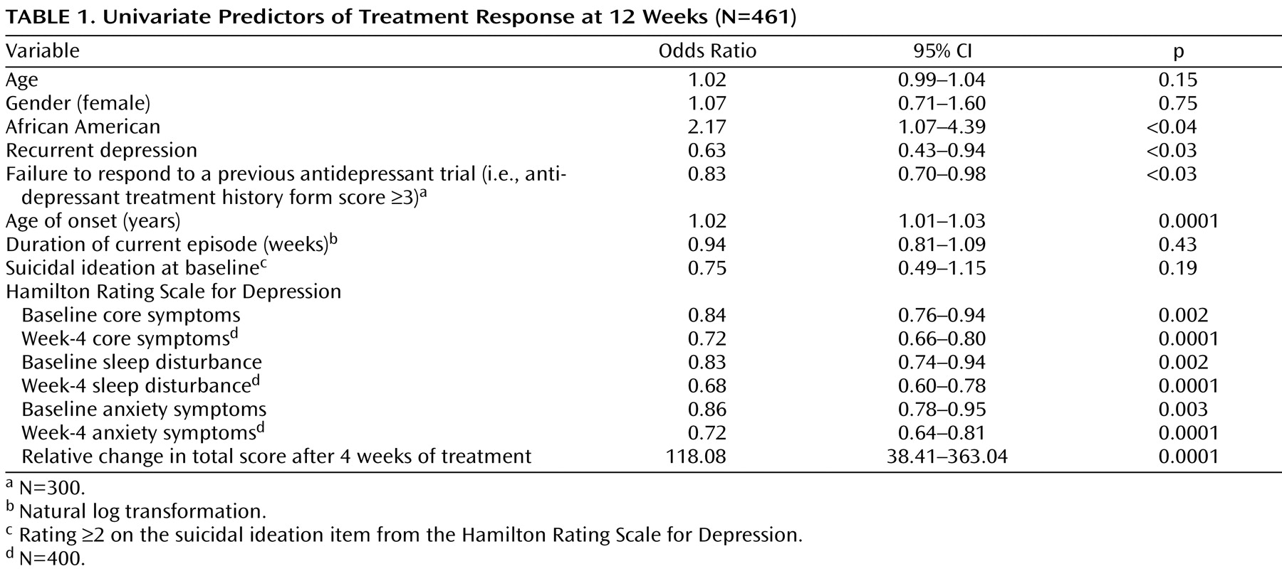
(28) . We initially performed a univariate logistic regression on the demographic and clinical variables to identify potential predictors of treatment response. Response at 12 weeks was the binary dependent variable (
Table 1 ). Subsequently, to obtain a hierarchy of these predictors, we incorporated these potential predictors in a receiver-operating characteristic model using signal detection theory as described by Kiernan at al
(29) .
Signal detection theory has been especially useful in analyses where predictors are likely to be highly collinear and interactions between independent variables exist
(29) . In our case, the signal is a binary outcome (response/nonresponse at 12 weeks) and the detection is for the set of predictor variables
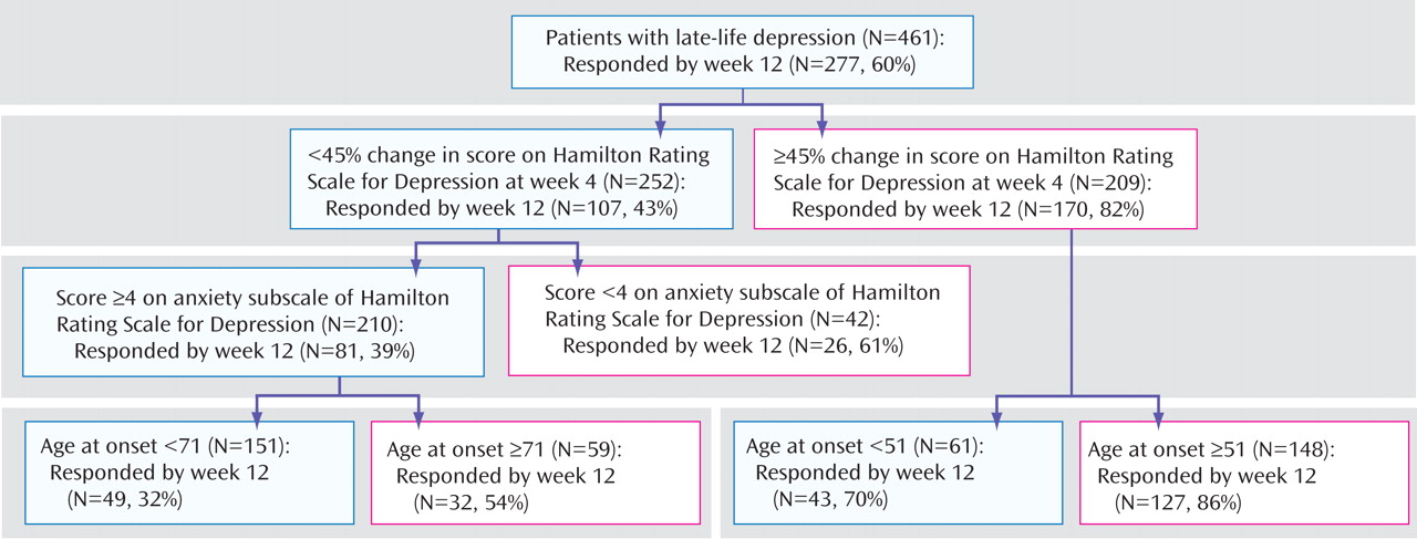
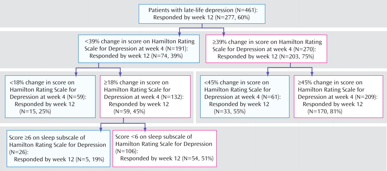
(29) . Signal detection identifies predictors with a stopping rule of p<0.05. The highest predicting variable is used to divide the sample into two subsamples, and the next predicting variable divides the higher-risk subsample. The process continues until the lowest risk variable stops at p<0.05
(29) . Variables associated with a p>0.05 are excluded from the decision tree. Signal detection determines the optimal cutoff point across all increments of a variable and across all variables
(29) .
We built two different models by modulating the sensitivity threshold for each predictor of treatment response to obtain hierarchies of risk correlated with different patients’ characteristics.
First, a low sensitivity threshold was used to define a model that minimizes false positives. A high rate of false positives (i.e., falsely predicting that patients will respond to treatment) could lead clinicians to continue a treatment that will eventually be ineffective. Avoiding this results in an aggressive treatment approach that clinicians might consider appropriate in various clinical situations (including but not limited to patients who have a higher risk of suicide or who are severely disabled by their depression).
Second, we used a high sensitivity threshold to define a model that minimizes false negatives. A high rate of false negatives (i.e., falsely predicting that a patient will be a nonresponder) could lead clinicians either to use unnecessary augmentation pharmacotherapy (thus exposing the patient to the risk of adverse effects) or to switch prematurely to another antidepressant (thus depriving patients from eventually responding to the first agent). Avoiding premature treatment changes results in a conservative approach (appropriate in various clinical situations, including but not limited to patients who have a history of multiple unsuccessful trials). In light of the results of the STAR-D study, emphasizing how long it can take to identify an effective treatment
(30,
31), it is important not to “miss” an effective treatment because of a premature switch.
For the first model (minimizing false positives), we used a sensitivity cutoff point of 0.3. For the second model (minimizing false negatives), we used a sensitivity cutoff point of 0.7
(32) . The selection of variables was based upon the univariate regression results and available sample. The potential predictors included race, age of onset, recurrence, baseline sleep disturbance, baseline anxiety, and early symptom improvement. Early symptom improvement was defined by the percent decrease in HAM-D score achieved by week 4. However, because clinicians do not use cutoff points such as those generated by the model, we converted the percentage cutoffs to corresponding clinical changes. Thus, we considered a decrease in HAM-D score of more than 45% at week 4 as a
marked early improvement, a decrease of HAM-D score between 30% and 45% as a
moderate early improvement, a decrease in HAM-D score between 18% and 30% as a
mild early improvement, and a decrease of HAM-D of less than 18% as the absence of clinically noticeable improvement, i.e., a
poor early improvement.
We used the antidepressant treatment history form to assess the adequacy of all the antidepressant trials received during the current episode based on both the duration and the dose of treatment. The antidepressant treatment history form scores are ordinal: 1 (definitely inadequate=trial of less than 4 weeks or of more than 4 weeks with a very low dose), 2 (probably inadequate=a trial of more than 4 weeks with probably inadequate doses), 3 (probably adequate=a trial of more than 4 weeks of an antidepressant at an adequate dose), 4 (definitely adequate=a trial longer than 4 weeks with intensive doses of antidepressant), or 5 (definitely adequate antidepressant with lithium augmentation). Antidepressant treatment history form scores were available for a subgroup of patients (N=289), and we repeated the analysis in this subgroup using the highest scores—corresponding to the strongest previous treatment trial the patient had failed to respond to during the current episode—as had been done in several previous analyses
(33,
34) .
