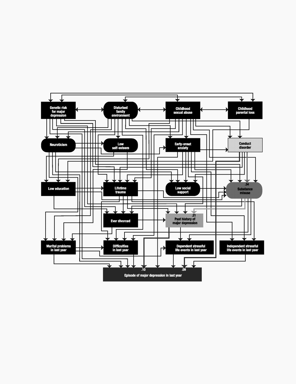
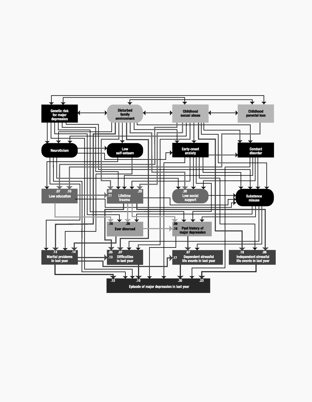
Model variables
The selection of variables began with those that had been used in our 1993 study (
30), which was based on data collected at FFQ, FF1, and FF2. Several of these variables could be improved with new information obtained in later waves. We had also collected information on several key variables lacking in our earlier model, especially childhood sexual abuse, conduct disorder, and substance misuse. Finally, we included other variables—based on the literature and their availability in our data—to expand the domains examined (e.g., self-esteem to include a “self-concept” variable and early-onset anxiety because of its strong demonstrated link to risk for subsequent major depression [
11]).
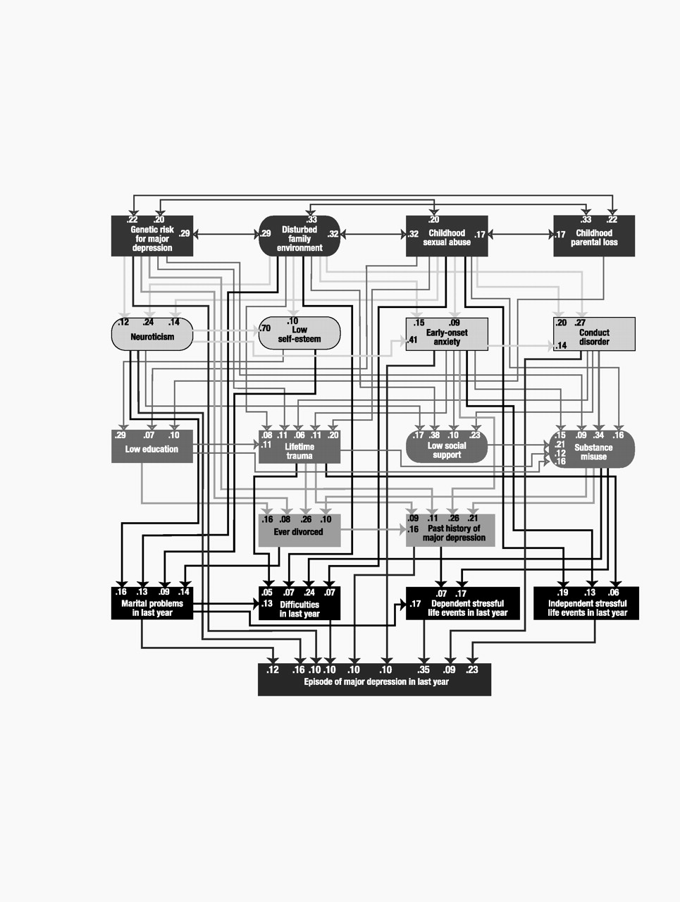
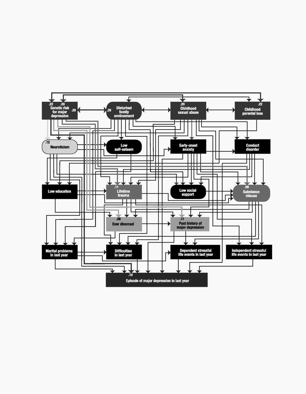
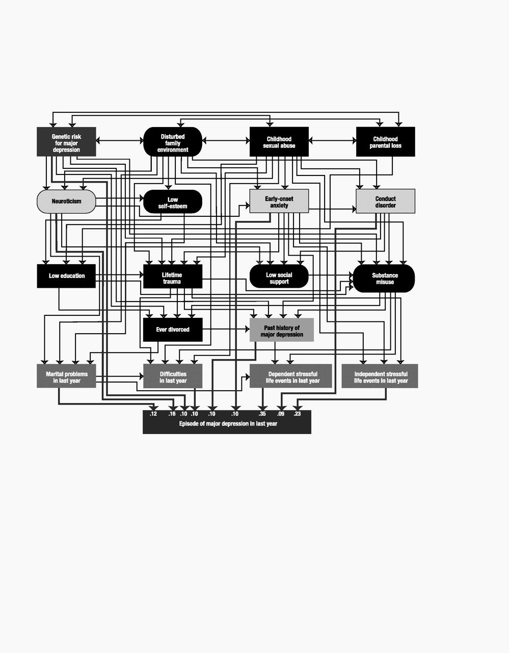
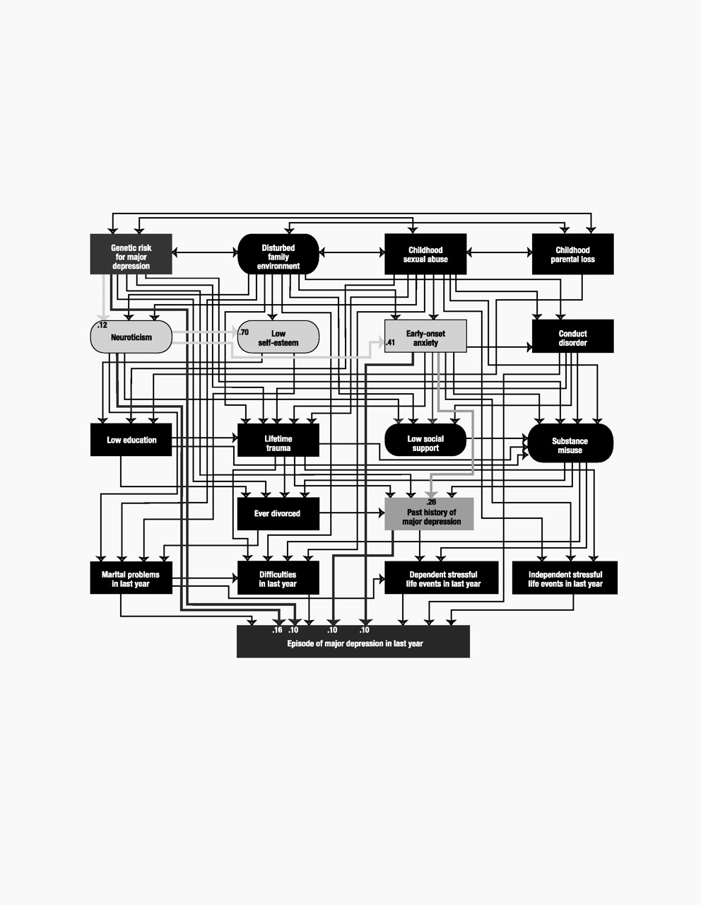
Our final list included 18 predictor variables that we attempted to order in a tentative developmental sequence. For ease of presentation, we organized these predictors into five “tiers” that roughly approximated five developmental periods: 1) childhood (genetic risk, disturbed family environment, childhood sexual abuse, and childhood parental loss), 2) early adolescence (neuroticism, self-esteem, and early-onset anxiety and conduct disorder), 3) late adolescence (educational attainment, lifetime traumas, social support, and substance misuse), 4) adulthood (history of divorce and past history of major depression), and 5) the last year (marital problems, difficulties, and stressful life events that were either dependent on or indepen-dent of the respondent’s own behavior). Of these 18 predictor variables, five were latent and were constructed, by using a measurement model, from other observed variables. We here outline briefly the nature of each variable.
Genetic risk was assessed by a composite measure of the lifetime history of major depression in the co-twin (assessed at FF1, FF3, and FF4) and in the mother and father (assessed in 1990–1991). Parents were divided into those who were affected and those who were unaffected. Co-twins were divided into four categories reflecting the number of interviews at which they received a diagnosis of lifetime major depression. To correct for varying base rates and degree of genetic relatedness in these relatives, we calculated the modified midrank score for the lifetime history of major depression and adjusted these scores to account for the varying genetic correlation with the proband twin (+1.00 for monozygotic co-twins and +0.50 for dizygotic co-twins and parents). We then took the mean of these three scores.
Disturbed family environment was assessed by a measurement model with two manifest continuous variables: mean parental warmth (measured with a modified version of the Parental Bonding Instrument [
33,
34]) and mean family environment score (measured by 14 items chosen from the Family Environment Scale [
35]). The Parental Bonding Instrument assessed parent-child relationships up to when the twins were age 16. The Family Environment Scale reflected the general emotional tone of the home when the twins “were growing up.” Mean parental warmth was calculated for each twin pair as the mean of the self-report and co-twin report of maternal and paternal warmth (assessed at FF2 and reversed-coded to reflect lack of warmth). For the family environment, we summed the items reflecting family tension (e.g., “family members would get so angry sometimes that they would throw things or hit each other”) and the reverse scoring of items reflecting family integration (e.g., “family members really helped and supported one another”). We then took the mean of the standardized scores of the twin and co-twin assessed at FF2 and the separately standardized score of mother and father assessed in 1990–1991. These four reports were then averaged and restandardized to create a single Family Environmental Scale score for the family.
Childhood sexual abuse was a binary variable based on twin self-report at FF4 (
36). Our previous analysis of these data (
37) suggested that the increased risk of major depression was associated largely with the more severe forms of abuse. Therefore, in these analyses, twins were assigned a score of 1 if they reported, before the age of 16, an unwanted sexual contact with an older individual that included “touching or fondling your private parts,” “making you touch them in a sexual way,” or “attempting or having sexual intercourse.” Validating the assessments of childhood sexual abuse is inherently problematic, but the agreement between self-report and co-twin-report in this sample far exceeded chance expectation (contingency coefficient=0.50, weighted kappa=0.40, 95% confidence interval [CI]=0.33–0.47).
Parental loss was a binary measure scored 1 if the twin reported that one or both parents left the nuclear home due to death, divorce, or parental separation before the twin was age 17. This was assessed with high reliability (98.5% agreement between twins [
38]).
Neuroticism was assessed with a measurement model utilizing the short (12-item) version of the Revised Eysenck Personality Questionnaire (
39) and data obtained at FFQ, FF1, and FF3. Because of the resulting J-shaped distribution, it was scored as a five-level ordinal measure.
Self-esteem was assessed with a measurement model based on the full Rosenberg Self-Esteem Scale (
40) by using data obtained at FF1 and FF3. Transformation was not needed because of the data’s symmetric distribution. This variable was reversed so that higher scores reflected lower self-esteem.
Early-onset anxiety disorder was a binary variable scored 1 for subjects with an onset before age 18 of panic disorder (data from FF1 or FF2), generalized anxiety disorder (data from FF1 or FF4), or phobia (data from FF1, FF2, or FF4). Panic disorder and generalized anxiety disorder were diagnosed with DSM-III-R criteria, except that we reduced the minimum duration of the latter disorder from 6 months to 1 month. Phobia was defined as the presence of an irrational fear that impacted in an objective and significant way on the behavior of the twin (
41).
Conduct disorder was treated as an ordinal variable that reflected the number of DSM-IV conduct disorder criteria met before age 18 that were endorsed at FF4.
The number of years of education was treated as a continuous variable, scored from 1 to 20 at the FF4 interview. It was reverse-scored to reflect low educational attainment.
The measure of lifetime traumas was based on data from FFQ and reflected the number of 10 possible items describing traumatic events that had ever occurred in the respondent’s lifetime, including physical assault, unexpected death of a loved one, and abortion. The distribution was skewed so that this measure was treated as an ordinal variable.
Social support was assessed by using a measurement model with information from the FF1 and FF3 interviews. We summed those dimensions of social support that related most strongly to risk for depression: problems with relatives and church and club attendance (
30). This measure, which was scored to reflect lack of social support, was relatively symmetric and was treated as a continuous variable.
Substance misuse was assessed with a measurement model derived from three binary manifest variables: 1) a lifetime diagnosis of DSM-III-R alcohol abuse or dependence assessed at FF3 or FF4, 2) a lifetime diagnosis of DSM-IV drug abuse or dependence at FF4 (separate assessments were made for cannabis, sedatives, stimulants, cocaine, opiates, hallucinogens, inhalants, and “over-the-counter” medications), and 3) lifetime nicotine dependence, assessed by a score of ≥7 on the Fagerstrom Tolerance Questionnaire (
42) for the period of heaviest smoking, by using data collected at FF3 or FF4.
Ever divorced was a binary measure scored 1 for women who reported a lifetime history of divorce at the FF1, FF3, or FF4 interviews. Never having been married was scored 0.
Prior history of major depression was a binary measure reflecting the presence or absence of a lifetime history of DSM-III-R major depression prior to 1 year before the FF1 interview (at the mean age of 28 years).
Marital problems in the last year was constructed as a three-level ordinal variable. In a piecewise regression that used seven items assessing the level of marital satisfaction in the last year from the Social Interaction Scale (
43), an elevated risk for onset of major depression was associated with levels of satisfaction in the lower 20%. Those who were unmarried or not living with a partner at FF4 were assigned an intermediate risk. Thus, the variable was constructed as follows: 0=upper 80% of marital satisfaction, 1=unmarried, and 2=lower 20% of marital satisfaction.
Difficulities in the last year, dependent stressful life events, and independent stressful life events were assessed by using our stressful life event measures. In the FF4 interview, each twin was systematically asked about the occurrence, at any time in the preceding 12 months, of 11 “personal” events (i.e., events occurring primarily to the informant): assault, divorce/separation, major financial problem, serious housing problems, serious illness or injury, job loss, legal problems, loss of confidant, serious marital problems, robbery, and serious difficulties at work. We also assessed four classes of “network” events: 1) serious trouble getting along with an individual in the network, 2) a serious personal crisis of someone in the network, 3) death of an individual in the network, and 4) serious illness of someone in the network. These events were presented separately for different relationships in their network (e.g., parents, siblings, offspring, etc.). Each reported event was dated to the nearest month with high interrater reliability (
44,
45). The dependence of a stressful life event, reflecting the probability that the respondent’s own behavior contributed to the stressful life event, was rated on a 4-point scale: clearly independent, probably independent, probably dependent, and clearly dependent, with demonstrated good interrater reliability (
46). In these analyses, we dichotomized stressful life events into those clearly or probably independent versus those clearly or probably dependent.
For an individual with a reported onset of major depression in the year preceding her FF4 interview, we counted, separately, the number of dependent and independent stressful life events occurring in that month and the 2 preceding months—the time period associated with an increased risk of depressive onset in this sample (
45). If the only episode occurred in the first or second month of the year (N=14), the number of stressful life events reported was multiplied, respectively, by 3 or 1.5. For individuals reporting no depressive onset, a random 3-month window was used to assess the occurrence of stressful life events. The number of stressful life events was treated as an ordinal variable. Difficulties in the last year reflected the sum of all stressful life events reported at other times during the year before the FF4 interview.
Statistical methods
Our structural equation model consisted of two parts: 1) a measurement model that consisted of factor loadings for the observed variables that index the five latent variables and 2) a structural model that consisted of path and correlation coefficients connecting the five latent and the 14 observed variables of the model proper. Model fitting was done by using Mplus, version 2 (
47), because of its ability to combine categorical, ordinal, and continuous data. The fit function was weighted least squares.
As in most longitudinal studies, missing data were a major problem. Excluding data from all subjects for whom one or more data points were missing would have resulted in unacceptable sample shrinkage. Therefore, the raw data was first put through multiple imputation by using IVEware (
48), which utilizes a multivariate sequential regression approach encompassing linear regression for continuous variables, Poisson regression for count variables (e.g., numbers of stressful life events, symptoms of conduct disorder), and logistic regression for ordinal and binary variables (
49). Five imputed data sets were created and then combined for analysis in Mplus, each being treated as one group in a multigroup analysis. The measurement model was not constrained across groups, and we did not attempt to simplify it in any way.
For the structural model, we began with a fully saturated model and used a combination of four approaches to produce a model with the optimal balance of explanatory power and parsimony. First, observing the significance levels of individual paths, we fixed sets of paths to zero when the associated z value was <1.96. Second, because our sample size was so large, some paths that remained significant were, in our judgment, too small to be meaningful. Therefore, our second step was to set all paths to zero with a value of <0.05, regardless of z value. In our third step, we further “trimmed” our model by setting paths to zero and looking for those where the increase in the model chi-square value was less than 3.84. As a last check, taking final results from an earlier iteration of the model, we added and subtracted a number of paths that were marginal by significance and/or magnitude to see if we could arrive at a better overall fit and indeed produced a modest improvement in fit and explanatory power.
We utilized three fit indices that reflect, in different ways, the success of the model in balancing explanatory power and parsimony: the Tucker-Lewis index (
50), the comparative fit index (
51), and the root mean square error of approximation (
52). For the Tucker-Lewis index and comparative fit index, values between 0.90 and 0.95 are considered acceptable and values ≥0.95 as good. For the root mean square error of approximation, good models have values ≤0.05, while values >0.10 are considered poor.
